Autoencoder reconstruction comparison

Compare the released MLP autoencoder with the mixed-baseline CNN on paired test examples. The published test split contains 3,066 PubMed, 79 Nilearn, and 202 NeuroVault maps. Because full PubMed reconstruction is slow on a typical Mac, this notebook evaluates the first 200 PubMed examples and the complete Nilearn and NeuroVault splits. Set DOMAIN_LIMITS["pubmed"] = None to run the complete PubMed test split. Set INCLUDE_FINETUNED = True only when you explicitly want the domain-fine-tuned CNN branches.

The provider downloads the published root-level split JSONLs and shared volume tensor from Hugging Face. Legacy local paths stored in individual JSONL rows are metadata only and are never loaded.

This is the paired_atlas_free protocol. Older PubMed MLP autoencoder comparisons loaded the MLP-native PubMed image resource and selected a different first-N cohort, while the CNN used atlas-free rows. Those older values are valid for their native cohort but are not expected to match this notebook. Here both families receive the same examples; the MLP bridge converts each shared volume to its established masker flat-map representation.

import matplotlib.pyplot as plt
import pandas as pd
import torch

from neurovlm import AtlasFreeCNNDataProvider, load_pipeline
from neurovlm.evaluation import (
    default_comparison_matrix,
    evaluate_reconstruction_comparison,
)

DOMAINS = ("pubmed", "nilearn", "neurovault")
DOMAIN_LIMITS = {
    "pubmed": 200,       # runtime-conscious default; use None for all 3,066
    "nilearn": None,     # complete test split: 79
    "neurovault": None,  # complete test split: 202
}
INCLUDE_FINETUNED = False  # explicit opt-in
DEVICE = "cuda" if torch.cuda.is_available() else "cpu"
EVALUATION_SCOPE = "PubMed first 200; Nilearn and NeuroVault complete test splits"

Run the comparison

The shared volume payload is about 4.2 GB and is downloaded once into the normal Hugging Face cache. Later providers reuse the cached payload.

results = []
for domain in DOMAINS:
    selections = default_comparison_matrix(
        "autoencoder",
        domains=(domain,),
        include_finetuned=INCLUDE_FINETUNED,
    )
    provider = AtlasFreeCNNDataProvider(
        domain=domain,
        limit=DOMAIN_LIMITS[domain],
    )
    results.append(evaluate_reconstruction_comparison(
        selections=selections,
        provider=provider,
        device=DEVICE,
    ))

summary = pd.DataFrame(row for result in results for row in result.summary)
by_source = pd.DataFrame(row for result in results for row in result.by_source)
by_sample = pd.DataFrame(row for result in results for row in result.by_sample)
manifest = pd.DataFrame(row for result in results for row in result.manifest)

summary.sort_values(["evaluation_domain", "family", "variant"])

	model_id	family	task	domain	variant	evaluation_domain	status	comparison_protocol	comparison_space	n	...	top10_overlap	top10_target_recall	top1_dice	top1_intersection_voxels	top1_overlap	top1_target_recall	top5_dice	top5_intersection_voxels	top5_overlap	top5_target_recall
5	cnn_autoencoder_mixed_baseline_eval_neurovault	cnn	autoencoder	None	mixed_baseline	neurovault	resolved	paired_atlas_free	native_atlas_free_volume	202	...	0.550961	0.550961	0.471101	290.198020	0.471101	0.471101	0.521068	1603.846535	0.521068	0.521068
4	mlp_autoencoder_eval_neurovault	mlp	autoencoder	None	default	neurovault	resolved	paired_atlas_free	mlp_masker_flatmap	202	...	0.213515	0.213515	0.064668	18.495050	0.064668	0.064668	0.132443	189.128713	0.132443	0.132443
3	cnn_autoencoder_mixed_baseline_eval_nilearn	cnn	autoencoder	None	mixed_baseline	nilearn	resolved	paired_atlas_free	native_atlas_free_volume	79	...	0.124388	0.124388	0.257377	158.544304	0.257377	0.257377	0.105070	323.405063	0.105070	0.105070
2	mlp_autoencoder_eval_nilearn	mlp	autoencoder	None	default	nilearn	resolved	paired_atlas_free	mlp_masker_flatmap	79	...	0.194471	0.194471	0.289944	82.924051	0.289944	0.289944	0.197807	282.468354	0.197807	0.197807
1	cnn_autoencoder_mixed_baseline_eval_pubmed	cnn	autoencoder	None	mixed_baseline	pubmed	resolved	paired_atlas_free	native_atlas_free_volume	200	...	0.505145	0.505145	0.609529	375.470000	0.609529	0.609529	0.575856	1772.485000	0.575856	0.575856
0	mlp_autoencoder_eval_pubmed	mlp	autoencoder	None	default	pubmed	resolved	paired_atlas_free	mlp_masker_flatmap	200	...	0.363461	0.363461	0.049703	14.215000	0.049703	0.049703	0.240700	343.720000	0.240700	0.240700

6 rows × 34 columns

Aggregate metric plots

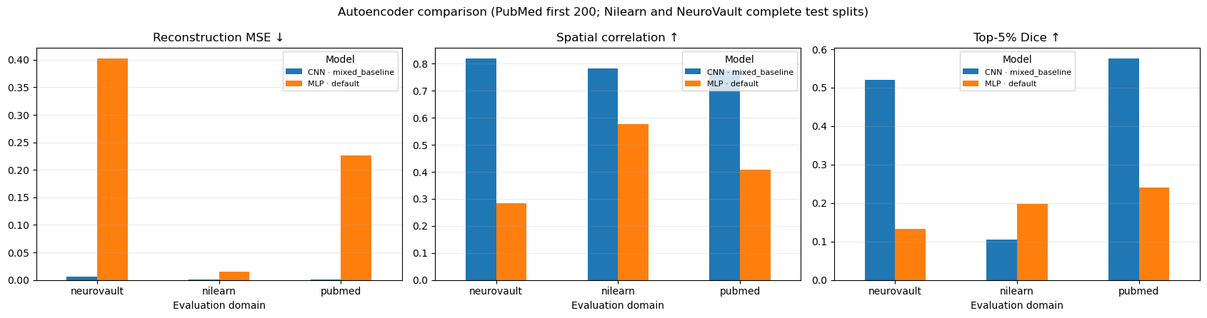
CNN metrics are computed in native atlas-free volume space; MLP metrics are computed in the established masker flat-map space. The plots compare complete pipelines in their declared spaces, not voxel-identical representations. Lower reconstruction MSE is better; higher spatial correlation and top-5% Dice are better.

resolved = summary[(summary["status"] == "resolved") & (summary["n"] > 0)].copy()
if resolved.empty:
    raise RuntimeError("No models resolved. Inspect `manifest` for checkpoint errors.")
resolved["model"] = resolved.apply(
    lambda row: f'{row["family"].upper()} · {row["variant"]}', axis=1
)

metrics = (
    ("reconstruction_mse", "Reconstruction MSE ↓"),
    ("spatial_corr", "Spatial correlation ↑"),
    ("top5_dice", "Top-5% Dice ↑"),
)
fig, axes = plt.subplots(1, len(metrics), figsize=(17, 4.5))
for ax, (metric, title) in zip(axes, metrics):
    table = resolved.pivot(index="evaluation_domain", columns="model", values=metric)
    table.plot.bar(ax=ax, rot=0)
    ax.set_title(title)
    ax.set_xlabel("Evaluation domain")
    ax.grid(axis="y", alpha=0.25)
    ax.legend(title="Model", fontsize=8)
fig.suptitle(f"Autoencoder comparison ({EVALUATION_SCOPE})")
fig.tight_layout()
plt.show()

Per-sample distributions

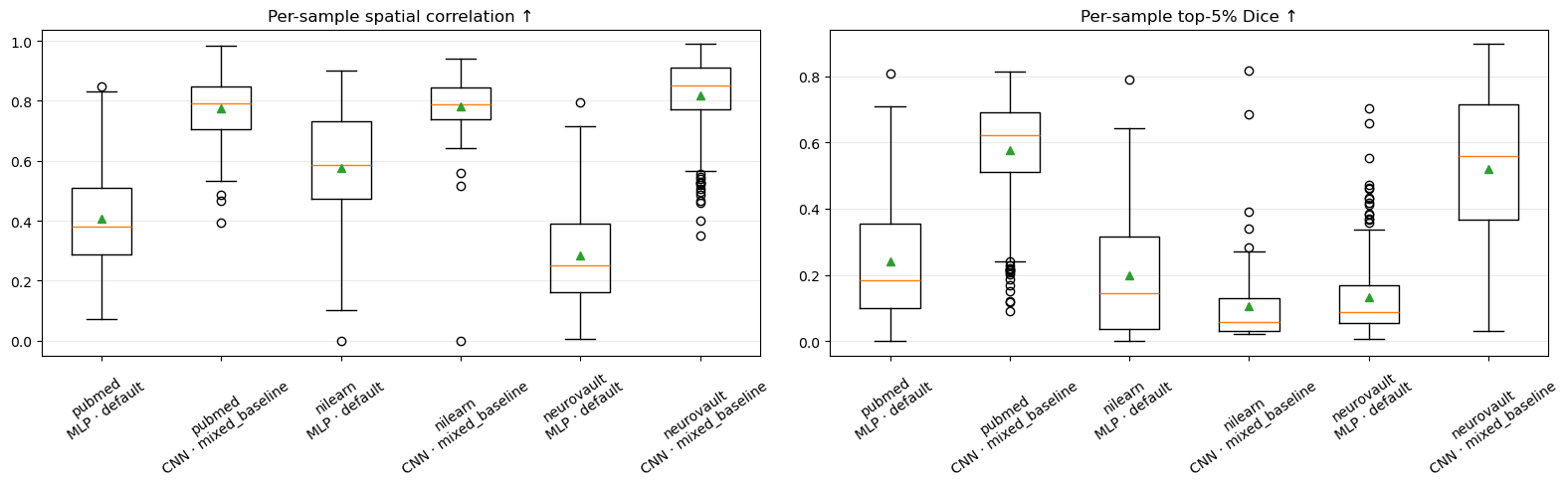
These box plots expose variance hidden by the aggregate means.

samples = by_sample.copy()
samples["model"] = samples.apply(
    lambda row: f'{row["family"].upper()} · {row["variant"]}', axis=1
)
samples["group"] = samples["evaluation_domain"] + "\n" + samples["model"]
group_names = list(dict.fromkeys(samples["group"]))

fig, axes = plt.subplots(1, 2, figsize=(16, 5))
for ax, metric, title in (
    (axes[0], "spatial_corr", "Per-sample spatial correlation ↑"),
    (axes[1], "top5_dice", "Per-sample top-5% Dice ↑"),
):
    values = [samples.loc[samples["group"] == name, metric].dropna() for name in group_names]
    ax.boxplot(values, labels=group_names, showmeans=True)
    ax.set_title(title)
    ax.tick_params(axis="x", labelrotation=35)
    ax.grid(axis="y", alpha=0.25)
fig.tight_layout()
plt.show()

/var/folders/vg/523p1fy95q907f9q2z7dz4880000gn/T/ipykernel_87627/1146578088.py:14: MatplotlibDeprecationWarning: The 'labels' parameter of boxplot() has been renamed 'tick_labels' since Matplotlib 3.9; support for the old name will be dropped in 3.11.
  ax.boxplot(values, labels=group_names, showmeans=True)
/var/folders/vg/523p1fy95q907f9q2z7dz4880000gn/T/ipykernel_87627/1146578088.py:14: MatplotlibDeprecationWarning: The 'labels' parameter of boxplot() has been renamed 'tick_labels' since Matplotlib 3.9; support for the old name will be dropped in 3.11.
  ax.boxplot(values, labels=group_names, showmeans=True)

Qualitative CNN reconstructions

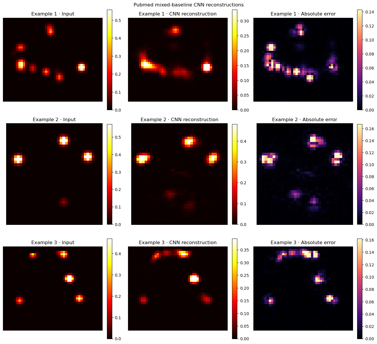
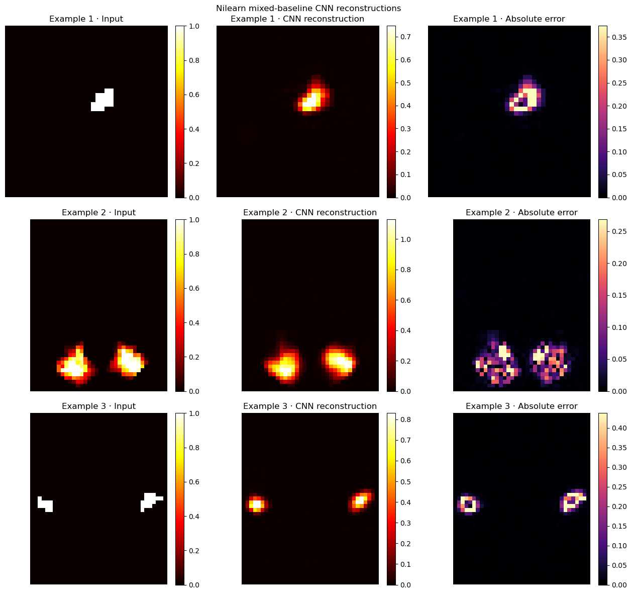
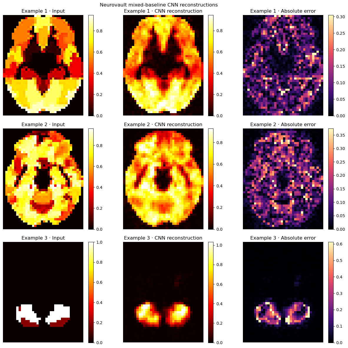
The next three cells show three examples per domain. All-zero maps are skipped—this matters for Nilearn because some very small atlas parcels disappear during 4 mm resampling/cropping. For every non-empty example, the sagittal, coronal, or axial plane with the greatest input activation is selected. Input, reconstruction, and error use independent robust color scales so sparse Nilearn parcels and lower-amplitude reconstructions remain visible; compare spatial structure rather than color magnitude across panels.

cnn = load_pipeline(family="cnn", task="autoencoder", device=DEVICE)
VISUAL_EXAMPLES_PER_DOMAIN = 3
PLANE_NAMES = ("sagittal", "coronal", "axial")

def _first_nonempty_examples(domain, count=VISUAL_EXAMPLES_PER_DOMAIN):
    data = AtlasFreeCNNDataProvider(domain=domain).test
    examples = []
    skipped = 0
    for index in range(len(data)):
        example = data[index]
        if int(torch.count_nonzero(example["volume"])) == 0:
            skipped += 1
            continue
        examples.append(example)
        if len(examples) == count:
            break
    if len(examples) != count:
        raise RuntimeError(f"Only {len(examples)} non-empty {domain} examples were available")
    return examples, skipped

def _strongest_plane(volume):
    candidates = []
    for axis, plane_name in enumerate(PLANE_NAMES):
        reduce_dims = tuple(dim for dim in range(3) if dim != axis)
        scores = volume.abs().sum(dim=reduce_dims)
        slice_index = int(scores.argmax())
        candidates.append((float(scores[slice_index]), axis, slice_index, plane_name))
    _, axis, slice_index, plane_name = max(candidates)
    return volume.select(axis, slice_index), axis, slice_index, plane_name

def _robust_positive_max(values):
    positive = values[values > 0]
    if not len(positive):
        return max(float(values.abs().max()), 1e-8)
    return max(float(torch.quantile(positive.float(), 0.99)), 1e-8)

def plot_reconstruction_domain(domain, count=VISUAL_EXAMPLES_PER_DOMAIN):
    examples, skipped = _first_nonempty_examples(domain, count)
    inputs = torch.stack([example["volume"] for example in examples])
    reconstructions = cnn.reconstruct(inputs).cpu()[:, 0]
    metadata = []
    fig, axes = plt.subplots(count, 3, figsize=(13, 4 * count))
    for row_index, (example, reconstruction) in enumerate(zip(examples, reconstructions)):
        truth = example["volume"][0].cpu()
        truth_plane, axis, slice_index, plane_name = _strongest_plane(truth)
        reconstruction_plane = reconstruction.select(axis, slice_index)
        error_plane = (reconstruction_plane - truth_plane).abs()
        panels = (
            (truth_plane, "Input", "hot"),
            (reconstruction_plane, "CNN reconstruction", "hot"),
            (error_plane, "Absolute error", "magma"),
        )
        for ax, (plane, title, cmap) in zip(axes[row_index], panels):
            image = ax.imshow(
                plane.T,
                origin="lower",
                cmap=cmap,
                vmin=0.0,
                vmax=_robust_positive_max(plane),
            )
            ax.set_title(f"Example {row_index + 1} · {title}")
            ax.axis("off")
            fig.colorbar(image, ax=ax, fraction=0.046, pad=0.04)
        metadata.append({
            "domain": domain,
            "example": row_index + 1,
            "map_id": example["map_id"],
            "plane": plane_name,
            "slice_index": slice_index,
            "all_zero_maps_skipped_before_selection": skipped,
        })
    fig.suptitle(f"{domain.title()} mixed-baseline CNN reconstructions")
    fig.tight_layout()
    plt.show()
    return pd.DataFrame(metadata)

PubMed: three reconstruction examples

plot_reconstruction_domain("pubmed")

	domain	example	map_id	plane	slice_index	all_zero_maps_skipped_before_selection
0	pubmed	1	pubmed_ale_34173239	sagittal	9	0
1	pubmed	2	pubmed_ale_23418930	coronal	15	0
2	pubmed	3	pubmed_ale_22634217	sagittal	18	0

Nilearn: three non-empty reconstruction examples

plot_reconstruction_domain("nilearn")

	domain	example	map_id	plane	slice_index	all_zero_maps_skipped_before_selection
0	nilearn	1	nilearn_schaefer_2018_392_7networks_rh_default...	coronal	13	1
1	nilearn	2	nilearn_juelich_probabilistic_51_gm_visual_cor...	axial	14	1
2	nilearn	3	nilearn_juelich_17_gm_inferior_parietal_lobule...	axial	24	1

NeuroVault: three reconstruction examples

plot_reconstruction_domain("neurovault")

	domain	example	map_id	plane	slice_index	all_zero_maps_skipped_before_selection
0	neurovault	1	neurovault_13877	axial	15	0
1	neurovault	2	neurovault_13883	axial	13	0
2	neurovault	3	neurovault_13894	axial	4	0